05 - Circuit Tools Graph Window
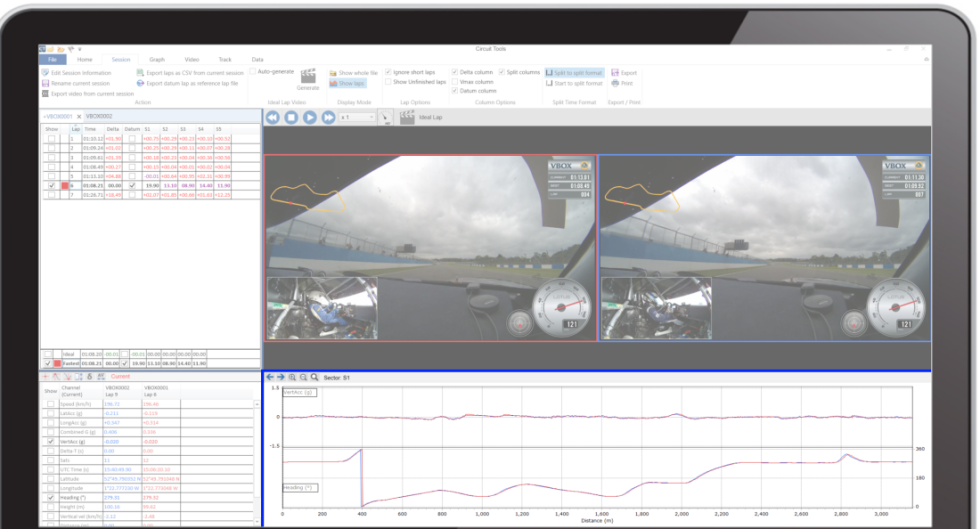
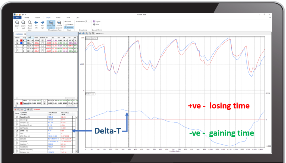
The graph window shows the logged channels in the form of a plot against distance, time or position. The speed channel is normally shown at the top.
The value of the channel at the cursor position is shown in the Data window. The data traces and channel values both use the same colour. By default the faster lap has a red trace. The current sector is also displayed for the selected location in the lap.
Zooming and Panning
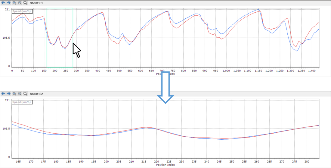
The quickest way to zoom in the Graph Window is to draw a zoom box with the left-hand mouse button from the left to the right. To zoom out, simply draw a box from the right to the left. You can also use the up and down arrow keys.
To pan, use the right-hand mouse button and drag the graph either way, or use CTRL and the cursor keys.
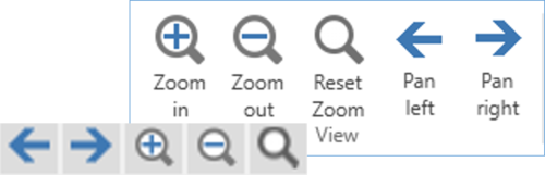
There are also buttons on the Graph Ribbon menu tab and just above the graph.
Delta-T (Lap-time difference)
The most useful parameter for comparing Laps is, by far, the Delta-T channel. Delta-T is the running lap time difference between two laps and it gives a very clear indication of where time is lost or gained around the circuit.
When the Delta-T is increasing, you are losing time, when it is decreasing, you are gaining time.
At first, look for the largest changes in Delta-T and concentrate on these areas.
Sometimes, in a corner, there may be a large gain followed by a large loss. This often happens when you enter a corner faster, but exit more slowly.
It is often surprising how much time you lose down the straight by exiting a corner a little bit slower than before.
|
Tip |
Graph Menu
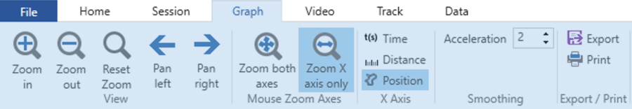
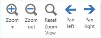
View
These buttons enable you to pan and zoom in the Graph window.
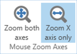
Mouse Zoom Axes
By default, the zoom only affects the X-axis. You can change this by using the buttons in the Graph Ribbon menu. By allowing zoom in both axes you can magnify the graph in more detail.
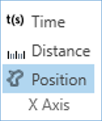
X-Axis
There are three ways of aligning comparison data: Time, Distance and Position. These are selectable via the Graph Ribbon menu. Position is the default X-axis and this is the method recommended for comparing two different laps. Time and distance are only used in special circumstances.
Traditionally, rolling distance has been used to align laps, but with the advantage of GPS it is better to use GPS position, as the distance travelled around a lap varies from lap to lap depending on the driving line. The position remains more accurate, as the error in GPS is much lower than the variation in rolling distance (which is often > 30m).
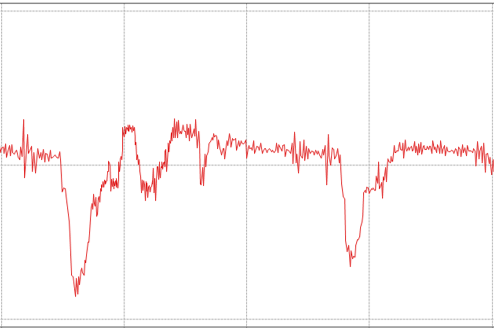
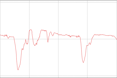
You can see a comparison of this effect below, from two different professional drivers at the Nordschleife during a race. The first plot uses the rolling distance to compare the two drivers, and the second uses GPS position. In the first plot, they have both travelled exactly 21060 m from the Start/Finish line, but they are 240 m apart! In the second plot, the GPS position of each vehicle is used to align the traces, and here you can see how closely they now line up.
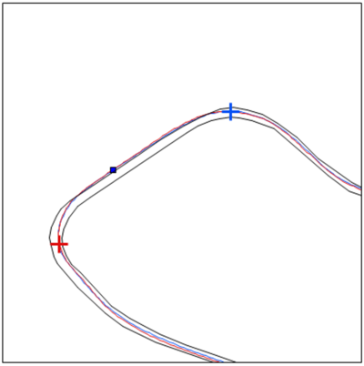 Distance alignment |
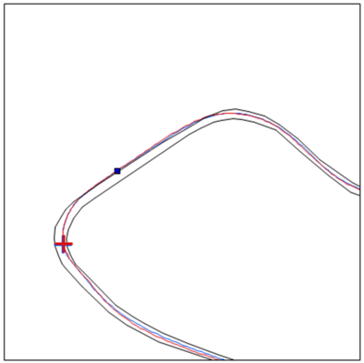 Position alignment |
Using GPS position alignment also makes the Delta-T value very accurate. This makes the values meaningful, even around the Nordschleife, where a Delta-T or predictive lap time based on distance would only be accurate to around 1 – 2 seconds after a full lap.
When using Position, the Delta-T and Predictive lap time are accurate to within 0.02 seconds around the full length of the Nordschleife!
Using Position to align laps
Note: Graphing using this method relies on good GPS position data. If you lose GPS position or you have heavy tree cover, then it is best to switch back to distance or even Time. If you leave the track, or cut out a part of the circuit, then again you will get a very poor position based comparison or you may even be unable to play the video or move the graph cursor beyond the point where you left the circuit if a poor datum is used.
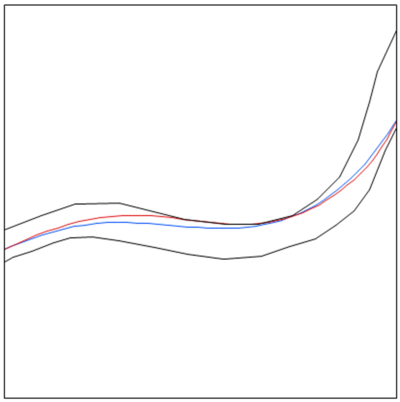
Smoothing
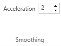
It is possible to change the level of smoothing applied to Acceleration channels, such as the lateral and longitudinal acceleration displayed in the Graph window. Applying higher levels of smoothing will produce a cleaner looking graph, however, it will also reduce the accuracy of the displayed results.
|
|
|
Export / Print
You can save the currently displayed graph view as an image file by selecting Export or print it by using the Print button.